4. Summary and diagnostics
Phil Bouchet, Enrico Pirotta, Catriona Harris, Len Thomas
Centre for Research into Ecological & Environmental Modelling, University of St Andrews2024-05-24
model_summary.RmdPreamble
This tutorial demonstrates how to inspect and summarize outputs from
the agent-based model within the narwind R package.
Viewing data
Outputs from the narw() simulator can be viewed in the R
console using the print() method. print() is
part of a group of generic R functions that can be applied to various R
objects and will behave differently depending on the type of object that
is passed to them. Other generic functions include plot(),
summary(), or write() (among others) – these
are covered in later sections.
print() can also be called ‘implicitly’, that is, by
simply typing the name of the relevant object in the R console and
pressing [Enter] on the keyboard. The default behavior for
objects returned by narw() is to give a tabular overview of
the data from the first 5 days of the simulation, and for the first
animal in each population cohort. For instance, to get a quick overview
of the outputs from the baseline_model created in the
previous tutorial, we can type:
model_baseOptional arguments allow users to override these default settings and
display data for specific days, animals, and/or cohorts, as needed. The
print() method has the following arguments:
| Argument | Default value | Description |
|---|---|---|
obj |
- |
Input model object returned by narw(). |
rowID |
1:5 |
Positive integer or vector of positive integers indicating which days of the simulation should be displayed. Defaults to the first first days. |
whale |
1 |
Positive integer indicating the individual for which data should be extracted. Only the first individual is included by default. |
cohort |
1:6 |
Positive integer or vector of positive integers indicating which
cohorts should be considered. Defaults to all cohorts. Cohort
identifiers are listed in an object called cohorts. Note
that calves are included with their mothers (i.e.,
cohort = 5). |
Given the above, the code below displays the first 5 days of the simulation for the fourth adult male.
print(model_base, rowID = 1:5, whale = 4, cohort = 3)
#>
#>
#>
#> =========================================================================================
#> Adults (male)
#> =========================================================================================
#>
#> --------------------------
#> Locations
#> --------------------------
#>
#>    whale day  date  easting northing region resid_m resid_sd pleave
#> 1:     4   1 01-10 685.5000 761.5000    SNE    20.4      1.1      0
#> 2:     4   2 02-10 684.7295 764.8358    SNE    20.4      1.1      0
#> 3:     4   3 03-10 687.2660 773.6351    SNE    20.4      1.1      0
#> 4:     4   4 04-10 683.5151 771.7780    SNE    20.4      1.1      0
#> 5:     4   5 05-10 689.2974 774.0483    SNE    20.4      1.1      0
#>
#> --------------------------
#> Attributes
#> --------------------------
#>    whale day cohort gsl seus alive      age        bc   length length_a
#> 1:     4   1      3   0    0     1 40.66953 0.3690396 13.62421 1362.755
#> 2:     4   2      3   0    0     1 40.67227 0.3692364 13.62422 1362.755
#> 3:     4   3      3   0    0     1 40.67501 0.3692556 13.62422 1362.755
#> 4:     4   4      3   0    0     1 40.67775 0.3693437 13.62422 1362.755
#> 5:     4   5      3   0    0     1 40.68049 0.3693518 13.62422 1362.755
#>    length_b length_c     mass leanmass  fatmass    mass_a   mass_b   mouth_r
#> 1:    -0.37    -0.18 29128.91 18379.19 10749.72 -4.834189 2.984353 0.1459854
#> 2:    -0.37    -0.18 29138.01 18379.20 10758.81 -4.834189 2.984353 0.1459854
#> 3:    -0.37    -0.18 29138.91 18379.20 10759.71 -4.834189 2.984353 0.1459854
#> 4:    -0.37    -0.18 29142.99 18379.21 10763.78 -4.834189 2.984353 0.1459854
#> 5:    -0.37    -0.18 29143.37 18379.22 10764.16 -4.834189 2.984353 0.1459854
#>    mouth_a  mouth_w abort starve died date_died p_surv
#> 1:    76.7 1.988936     0      0    0         0      1
#> 2:    76.7 1.988936     0      0    0         0      1
#> 3:    76.7 1.988936     0      0    0         0      1
#> 4:    76.7 1.988936     0      0    0         0      1
#> 5:    76.7 1.988937     0      0    0         0      1
#>
#> --------------------------
#> Stressors
#> --------------------------
#>
#>    whale day gear_risk is_entgl entgl_head entgl_sev entgl_d entgl_start
#> 1:     4   1         0        0          0         0       0           0
#> 2:     4   2         0        0          0         0       0           0
#> 3:     4   3         0        0          0         0       0           0
#> 4:     4   4         0        0          0         0       0           0
#> 5:     4   5         0        0          0         0       0           0
#>    entgl_end is_entgl_calf entgl_head_calf entgl_sev_calf entgl_d_calf
#> 1:         0             0               0              0            0
#> 2:         0             0               0              0            0
#> 3:         0             0               0              0            0
#> 4:         0             0               0              0            0
#> 5:         0             0               0              0            0
#>    entgl_start_calf entgl_end_calf strike_risk strike strike_calf noise_resp
#> 1:                0              0           0      0           0          0
#> 2:                0              0           0      0           0          0
#> 3:                0              0           0      0           0          0
#> 4:                0              0           0      0           0          0
#> 5:                0              0           0      0           0          0
#>    noise_lvl dB_thresh
#> 1:         0         0
#> 2:         0         0
#> 3:         0         0
#> 4:         0         0
#> 5:         0         0
#>
#> --------------------------
#> Activity budgets
#> --------------------------
#>
#>    whale day d_travel swimspeed      glide glide_feed glide_echelon t_travel
#> 1:     4   1 3.423671 0.7599443 0.08832360  0.2232512             0 1.251433
#> 2:     4   2 9.157525 1.1813921 0.08533398  0.2958658             0 2.153186
#> 3:     4   3 4.185526 0.8862305 0.08746686  0.5911404             0 1.311900
#> 4:     4   4 6.212131 0.7800888 0.08805436  0.4770002             0 2.212046
#> 5:     4   5 7.392055 1.0094592 0.08695322  0.2709297             0 2.034108
#>      t_feed t_rest_nurse
#> 1: 16.26587     6.482699
#> 2: 15.69783     6.148987
#> 3: 16.76200     5.926096
#> 4: 16.56145     5.226507
#> 5: 15.23622     6.729675
#>
#> --------------------------
#> Growth
#> --------------------------
#>
#>    whale day  delta_fat  EDlip EDpro lip_anab lip_catab perc_muscle
#> 1:     4   1 10.1698638 39.539 23.64      0.8       0.8   0.5537975
#> 2:     4   2  9.0891762 39.539 23.64      0.8       0.8   0.5537975
#> 3:     4   3  0.8916973 39.539 23.64      0.8       0.8   0.5537975
#> 4:     4   4  4.0747901 39.539 23.64      0.8       0.8   0.5537975
#> 5:     4   5  0.3762128 39.539 23.64      0.8       0.8   0.5537975
#>    perc_viscera perc_bones
#> 1:    0.2009494  0.2452532
#> 2:    0.2009494  0.2452532
#> 3:    0.2009494  0.2452532
#> 4:    0.2009494  0.2452532
#> 5:    0.2009494  0.2452532
#>
#> --------------------------
#> Energy balance
#> --------------------------
#>
#>    whale day     E_tot      E_in    E_out
#> 1:     4   1 502.63280  990.0397 487.4069
#> 2:     4   2 449.22117 1002.6947 553.4736
#> 3:     4   3  44.07103  534.0915 490.0205
#> 4:     4   4 201.39141  696.4399 495.0485
#> 5:     4   5  18.59385  552.1606 533.5668
#>
#> --------------------------
#> Energy intake
#> --------------------------
#>
#>    whale day feed preyconc   minprey     gape feedspeed captEff impedance
#> 1:     4   1    1 3.886321 0.4686015 2.676211 0.7599443 0.91575         0
#> 2:     4   2    1 2.631467 0.4686015 2.676212 1.1813921 0.91575         0
#> 3:     4   3    1 1.754626 0.4686015 2.676213 0.8862305 0.91575         0
#> 4:     4   4    1 2.631467 0.4686015 2.676214 0.7800888 0.91575         0
#> 5:     4   5    1 1.754626 0.4686015 2.676215 1.0094592 0.91575         0
#>    feed_effort eta_lwrBC eta_upprBC  targetBC    cop_mass     cop_kJ digestEff
#> 1:   0.4904317        10         30 0.3674076 0.001670151 0.02391922      0.94
#> 2:   0.4889457        10         30 0.3674076 0.001670151 0.02391922      0.94
#> 3:   0.4876203        10         30 0.3674076 0.001670151 0.02391922      0.94
#> 4:   0.4874909        10         30 0.3674076 0.001670151 0.02391922      0.94
#> 5:   0.4868979        10         30 0.3674076 0.001670151 0.02391922      0.94
#>    metabEff_juv metabEff_ad       E_cop
#> 1:    0.7403977       0.875 0.004762958
#> 2:    0.7403977       0.875 0.004762958
#> 3:    0.7403977       0.875 0.004762958
#> 4:    0.7403977       0.875 0.004762958
#> 5:    0.7403977       0.875 0.004762958
#>
#> --------------------------
#> Energetic costs
#> --------------------------
#>
#>    whale day    E_out      rmr       LC scalar_LC     stroke stroke_feed
#> 1:     4   1 487.4069 461.2304 26.07615         1 0.10982960   0.1609924
#> 2:     4   2 553.4736 461.2305 92.14276         1 0.14646990   0.1678607
#> 3:     4   3 490.0205 461.2307 28.68960         1 0.09891408   0.1725391
#> 4:     4   4 495.0485 461.2308 33.71755         1 0.07163653   0.1636737
#> 5:     4   5 533.5668 461.2309 72.23578         1 0.14700101   0.1642192
#>     E_growth
#> 1: 0.1003045
#> 2: 0.1002551
#> 3: 0.1002057
#> 4: 0.1001564
#> 5: 0.1001070
Note 4.1: The
print()method is only used for viewing data inside the R console. To export / save data on disk, use theexport()method (see relevant tutorial).
Model summary and diagnostics
The summary() method provides a range of diagnostics
that are helpful for assessing whether simulated whale behavior aligns
with biological expectations. These relate to individual (1) health, (2)
movements, (3) habitat use, (4) behavior (i.e., activity budgets), (5)
stressor exposure, and (6) energy intake vs. expenditure (see Table 1
below).
The function takes the following arguments:
| Argument | Default value | Description |
|---|---|---|
obj |
- |
Model object of class narwsim, as returned by
narw(). |
what |
"all" |
Character string indicating which component(s) of the summary to
display. Can be one of: "health", "movements",
"habitat", "behavior",
"stressors", "strike", "gear",
"noise", "other", or "energy".
See below for details. Defaults to "all" for a complete
summary. |
relative |
FALSE |
Logical. If TRUE, percentages are calculated relative
to class totals. Defaults to FALSE. |
quintile |
TRUE |
Logical. If TRUE, body condition plots (under the
“health” section) are based on quintiles of the data. |
plot |
FALSE |
Logical. If TRUE, plots are produced in addition to a
text-based summary. |
whale |
1:nsim |
Positive integer indicating the individual for which data should be
extracted. By default, considers all nsim individuals. |
cohort |
1:6 |
Positive integer or vector of positive integers indicating which
cohorts should be considered. Defaults to all cohorts. Cohort
identifiers are listed in an object called cohorts. |
As summaries tend to be long and dense, the what
argument can be used to select subsets of data to show in the R console.
The table below lists the information returned for each possible value
of what.
| Category | Component | Plots | Details |
|---|---|---|---|
health |
Mortality | No | Whale mortality by region, cohort, and cause of death (i.e., starvation vs. vessel strike) . |
| Pregnancy | No | Observed abortion rate in females that started the simulation in a pregnant state. | |
| Births | No | Mean (range) date of calving events. | |
| Body condition | Yes | Time series of individual body condition (expressed as relative fat mass), by cohort. | |
| Growth | Yes | Growth curves, by cohort. | |
movements |
Locations | No | Breakdown of (daily) locations by cohort, region, and country (U.S. vs. Canada). |
| Destinations | No | Comparison of assigned vs. realized migratory destinations both within and across cohorts. Migratory endpoints include the Southeastern United States calving grounds (SEUS) and Canadian feeding grounds in the Gulf of St Lawrence (GSL). | |
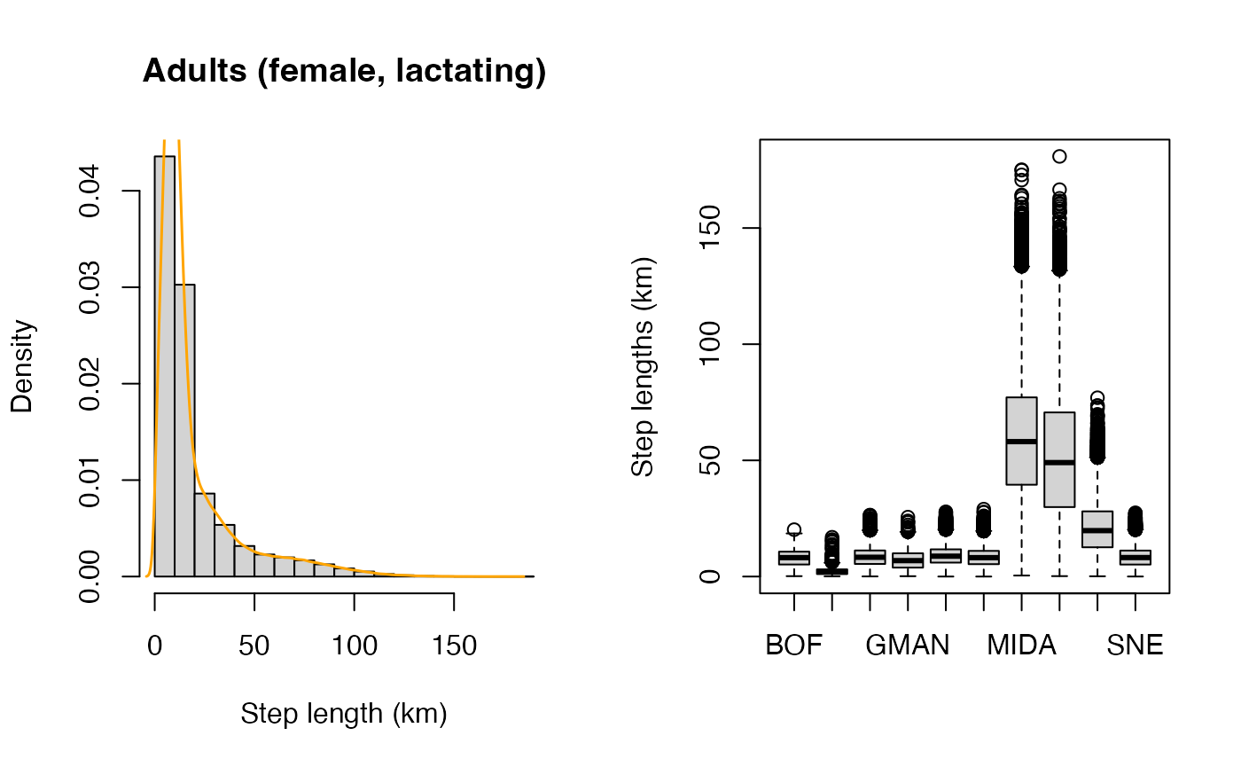
| Step lengths | Yes | Summary of daily movements, reported as mean (± SD, range) distances traveled per day, by cohort. Distributions of daily step lengths are also visualized by region and as a whole. | |
| Migration | No | Summary of yearly movements, reported as mean (± SD, range) total distance covered over the time span of the simulation, by cohort. | |
habitat |
Occupancy | No | Cohort-specific summary of the numbers of animals visiting each region, and the number of regions visited by animals. |
| Residency | No | Breakdown of days spent in each. | |
behavior |
Activity budgets | Yes | Mean (± SD) hours spent engaging in each of the four categories of behavior considered in the model (i.e., traveling, resting, nursing, and feeding), by region. A visual breakdown by region is also produced for each category of behavior. |
stressors |
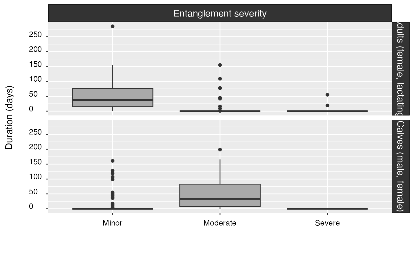
Entanglements (gear) |
Yes | Various summaries by cohort, including: entanglement rates, durations, severities, probabilities, and attachment sites along the body. |
Vessel strikes (strike) |
No | Strike rates by cohort. | |
Noise (noise) |
No | Summary of mean (± SD, range) noise levels encountered, behavioral response thresholds, and numbers of days during which a response to pile-driving was observed. | |
Other sources of mortality (other) |
No | Summary of mortality from other sources, by cohort. | |
| Energy | Energy budget | No | Mean (± SD, range) daily energy intake and expenditure (expressed in MJ/day), by cohort. Also reported are the mean (± SD, range) % time individuals are in energetic deficit (energy balance < 0) or surplus (energy balance > 0). |
Similarly, the cohort argument can be used to only
display data for specific population cohorts. This works based on a
unique cohort ID number, which is an integer between 1 and 6. A list of
cohort IDs is stored in the left-most column of an object called
cohorts, as shown below:
cohorts
#>    id                       name     class     abb  colour
#> 1:  0      Calves (male, female)    Calves  c(m,f)   black
#> 2:  1           Juveniles (male) Juveniles  jv(ml) #104E8B
#> 3:  2         Juveniles (female) Juveniles jv(fml) #F69554
#> 4:  3              Adults (male)    Adults  ad(ml) #22BA9C
#> 5:  4  Adults (female, pregnant)    Adults ad(f,p) #84375A
#> 6:  5 Adults (female, lactating)    Adults ad(f,l) #EEB422
#> 7:  6   Adults (female, resting)    Adults ad(f,r) #942F33
Based on this, the code below prints a complete summary (all categories of data listed in the above table) for the cohorts of lactating (ID = 5) females:
# Summary for adult females only
summary(model_base, cohort = 5)
#> -------------------------------------------------------------
#> -------------------------------------------------------------
#>
#>      NORTH ATLANTIC RIGHT WHALE (Eubalaena glacialis)
#>
#>              *** PCoMS MODEL SUMMARY ***
#>
#> -------------------------------------------------------------
#> -------------------------------------------------------------
#>
#> BOF: Bay of Fundy
#> CCB: Cape Cod Bay
#> CST: Cabot Strait
#> GMAN: Grand Manan Basin
#> GOM: Gulf of Maine and Georges Bank
#> GSL: Gulf of St Lawrence
#> MIDA: Mid-Atlantic
#> SCOS: Scotian Shelf
#> SEUS: Southeastern United States
#> SNE: Southern New England
#>
#> =============================================================
#> SIMULATIONS
#> =============================================================
#>
#> No. animals: 1,000
#>
#> Cohort(s)
#> ----------
#> c(m,f): Calves (male, female)
#> ad(f,l): Adults (female, lactating)
#>
#> Simulation start: October
#>
#> =============================================================
#> HEALTH
#> =============================================================
#>
#> +++++++++++ Mortality +++++++++++
#>
#> cohort                       alive         dead
#> ---------------------------  ------------  ------------
#> Adults (female, lactating)   92.4% (924)   7.6%  (76)
#> Calves (male, female)        82.6% (826)   17.4% (174)
#>
#> +++++++++++ Mortality (by source) +++++++++++
#>
#> cohort    cause_death        N
#> --------  -----------------  ----------
#> ad(f,l)   starve             4.5% (45)
#> ad(f,l)   natural            1.8% (18)
#> ad(f,l)   strike             1.3% (13)
#> c(m,f)    starve             8.2% (82)
#> c(m,f)    natural            2.7% (27)
#> c(m,f)    starve (female)    2.7% (27)
#> c(m,f)    natural (female)   1.7% (17)
#> c(m,f)    strike (female)    1.2% (12)
#> c(m,f)    strike             0.9%  (9)
#>
#> +++++++++++ Mortality (by region) +++++++++++
#>
#> region   cause_death   ad(f,l)     c(m,f)
#> -------  ------------  ----------  ----------
#> CST      natural       0.0%  (0)   0.6%  (1)
#> GOM      natural       3.9%  (3)   4.0%  (7)
#> GSL      natural       3.9%  (3)   1.1%  (2)
#> MIDA     natural       1.3%  (1)   0.6%  (1)
#> SCOS     natural       2.6%  (2)   2.9%  (5)
#> SEUS     natural       9.2%  (7)   4.6%  (8)
#> SNE      natural       2.6%  (2)   1.7%  (3)
#>
#>
#> region   cause_death        ad(f,l)     c(m,f)
#> -------  -----------------  ----------  ----------
#> GOM      natural (female)   0.0%  (0)   1.7%  (3)
#> GSL      natural (female)   0.0%  (0)   1.7%  (3)
#> MIDA     natural (female)   0.0%  (0)   0.6%  (1)
#> SCOS     natural (female)   0.0%  (0)   1.1%  (2)
#> SEUS     natural (female)   0.0%  (0)   4.0%  (7)
#> SNE      natural (female)   0.0%  (0)   0.6%  (1)
#>
#>
#> region   cause_death   ad(f,l)      c(m,f)
#> -------  ------------  -----------  -----------
#> CCB      starve        1.3%  (1)    0.0%  (0)
#> CST      starve        13.2% (10)   7.5% (13)
#> GMAN     starve        1.3%  (1)    1.1%  (2)
#> GOM      starve        6.6%  (5)    12.6% (22)
#> GSL      starve        3.9%  (3)    2.9%  (5)
#> MIDA     starve        2.6%  (2)    3.4%  (6)
#> SCOS     starve        13.2% (10)   18.4% (32)
#> SNE      starve        17.1% (13)   1.1%  (2)
#>
#>
#> region   cause_death       ad(f,l)     c(m,f)
#> -------  ----------------  ----------  ----------
#> CST      starve (female)   0.0%  (0)   1.7%  (3)
#> GMAN     starve (female)   0.0%  (0)   0.6%  (1)
#> GOM      starve (female)   0.0%  (0)   2.9%  (5)
#> GSL      starve (female)   0.0%  (0)   0.6%  (1)
#> MIDA     starve (female)   0.0%  (0)   1.1%  (2)
#> SCOS     starve (female)   0.0%  (0)   5.2%  (9)
#> SNE      starve (female)   0.0%  (0)   3.4%  (6)
#>
#>
#> region   cause_death   ad(f,l)     c(m,f)
#> -------  ------------  ----------  ----------
#> GMAN     strike        0.0%  (0)   0.6%  (1)
#> GOM      strike        1.3%  (1)   0.0%  (0)
#> GSL      strike        1.3%  (1)   0.0%  (0)
#> MIDA     strike        0.0%  (0)   0.6%  (1)
#> SEUS     strike        6.6%  (5)   2.9%  (5)
#> SNE      strike        7.9%  (6)   1.1%  (2)
#>
#>
#> region   cause_death       ad(f,l)     c(m,f)
#> -------  ----------------  ----------  ----------
#> GOM      strike (female)   0.0%  (0)   0.6%  (1)
#> GSL      strike (female)   0.0%  (0)   0.6%  (1)
#> SEUS     strike (female)   0.0%  (0)   2.9%  (5)
#> SNE      strike (female)   0.0%  (0)   2.9%  (5)
#>
#>
#> +++++++++++ Births +++++++++++
#>
#> No. births: 1000 (100%)
#> DOB: 1 Jan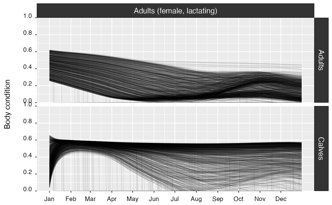
#>
#> =============================================================
#> MOVEMENTS (km)
#> =============================================================
#>
#> +++++++++++ Migratory destinations (by cohort) +++++++++++
#>
#> cohort    SEUS   reach_not   reach
#> --------  -----  ----------  --------------
#> ad(f,l)   0      0.0% (0)    100.0%  (947)
#> ad(f,l)   1      0.0% (0)    100.0% (1000)
#>
#>
#> cohort    GSL   reach_not      reach
#> --------  ----  -------------  ------------
#> ad(f,l)   0     86.5% (1038)   13.5% (162)
#> ad(f,l)   1     5.1%   (38)    94.9% (709)
#>
#> +++++++++++ Migratory destinations (all individuals) +++++++++++
#>
#> SEUS   reach_not   reach
#> -----  ----------  --------------
#> 0      0.0% (0)    100.0%  (947)
#> 1      0.0% (0)    100.0% (1000)
#>
#>
#> GSL   reach_not      reach
#> ----  -------------  ------------
#> 0     86.5% (1038)   13.5% (162)
#> 1     5.1%   (38)    94.9% (709)
#>
#> +++++++++++ Step lengths and migration distances +++++++++++
#>
#> cohort    step                   migration
#> --------  ---------------------  ------------------------------
#> ad(f,l)   18.9 (±21) [0–180.8]   8,516 (±1,052) [2,186–11,895]
#>
#> =============================================================
#> HABITAT USE
#> =============================================================
#>
#> region   ad(f,l)
#> -------  ---------------
#> BOF      0.1%    (351)
#> CCB      0.1%    (442)
#> CST      4.9%  (21970)
#> GMAN     0.8%   (3459)
#> GOM      20.9%  (92730)
#> GSL      9.4%  (41809)
#> MIDA     8.5%  (37875)
#> SCOS     7.4%  (32939)
#> SEUS     23.3% (103702)
#> SNE      24.6% (109103)
#>
#>
#> country   ad(f,l)
#> --------  ---------------
#> Canada    22.6% (100528)
#> U.S.      77.4% (343852)
#>
#> +++++++++++ Number of animals visiting each region (N = 1000) +++++++++++
#>
#> region   ad(f,l)
#> -------  ------------
#> BOF      2.9% (29)
#> CCB      0.8% (8)
#> CST      56.3% (563)
#> GMAN     13.9% (139)
#> GOM      98.2% (982)
#> GSL      43.7% (437)
#> MIDA     100% (1000)
#> SCOS     94.3% (943)
#> SEUS     100% (1000)
#> SNE      100% (1000)
#>
#> +++++++++++ Days spent in each region +++++++++++
#>
#> region   ad(f,l)
#> -------  -----------------------
#> BOF      12.1 (±9.4) [1–34]
#> CCB      55.2 (±52.6) [5–130]
#> CST      39 (±14.9) [2–93]
#> GMAN     24.9 (±14.1) [1–92]
#> GOM      94.4 (±49.1) [1–245]
#> GSL      95.7 (±42.2) [1–180]
#> MIDA     37.9 (±9.9) [13–136]
#> SCOS     34.9 (±19.4) [1–114]
#> SEUS     104.1 (±14.5) [45–146]
#> SNE      109.1 (±37.5) [34–313]
#>
#> +++++++++++ Total number of regions visited +++++++++++
#>
#>  No.regions  ad(f,l)
#> -----------  -------------
#>           3  100.0%  (18)
#>           4  100.0%  (39)
#>           5  100.0% (278)
#>           6  100.0% (173)
#>           7  100.0% (474)
#>           8  100.0%  (17)
#>           9  100.0%   (1)
#>
#> =============================================================
#> ACTIVITY BUDGETS
#> =============================================================
#>
#> +++++++++++  Adults (female, lactating)  +++++++++++
#>
#> region   travel (hrs)    rest/nurse (hrs)   feed (hrs)
#> -------  --------------  -----------------  --------------
#> SNE      4.64 (±4.02)    12.52 (±6.93)      16.11 (±0.62)
#> MIDA     15.56 (±6.01)   7.68 (±6.16)       7.44 (±5.45)
#> SEUS     11.61 (±5.81)   12.39 (±5.81)      0 (± 0)
#> GOM      3.3 (±2.4)      6.57 (±4.65)       16.11 (±0.64)
#> SCOS     14.46 (±6.47)   1.33 (±3.27)       8.87 (±5.59)
#> CCB      1.61 (±1.58)    20.1 (±5.92)       16.07 (±0.66)
#> GMAN     2.71 (±2.12)    8.48 (±6.53)       16.11 (±0.61)
#> CST      3.18 (±2.35)    7.42 (±5.6)        16.11 (±0.64)
#> GSL      2.72 (±1.56)    5.59 (±3.04)       16.11 (±0.63)
#> BOF      2.62 (±1.52)    5.5 (±2.33)        16.11 (±0.64)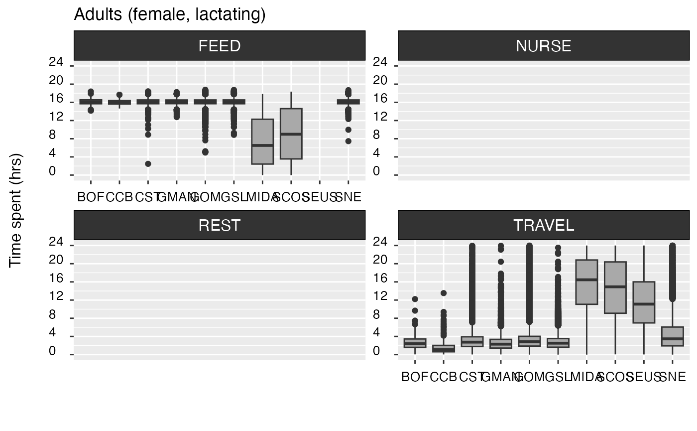
#>
#> =============================================================
#> STRESSORS
#> =============================================================
#>
#> +++++++++++ Entanglements +++++++++++
#>
#> entangled   rate
#> ----------  -------------
#> no          91.2% (1825)
#> yes         8.8% (175)
#>
#>
#> position   rate
#> ---------  -----------
#> body       51.4% (90)
#> head       48% (84)
#> head       0.6% (1)
#>
#>
#> cohort    not entangled   entangled
#> --------  --------------  ----------
#> ad(f,l)   91.0% (910)     9.0% (90)
#> c(m,f)    91.5% (915)     8.5% (85)
#>
#>
#> cohort    No. events per animal   p(entangled)
#> --------  ----------------------  ---------------------
#> ad(f,l)   1.06 (±0.27) [1–3]      0 (±0.002) [0–0.217]
#> c(m,f)    1 (±0) [1–1]            NA
#>
#>
#> cohort    minor        moderate     severe
#> --------  -----------  -----------  ---------
#> ad(f,l)   87.9% (80)   9.9%  (9)    2.2% (2)
#> c(m,f)    18.8% (16)   81.2% (69)   0.0% (0)
#>
#>
#> cohort    minor (days)       moderate (days)    severe (days)
#> --------  -----------------  -----------------  -----------------
#> ad(f,l)   57 (±46) [1–285]   59 (±51) [1–155]   37 (±25) [19–55]
#> c(m,f)    59 (±49) [4–161]   60 (±46) [4–199]   0 (±0) [0–0]
#>
#>
#> +++++++++++ Vessel strikes +++++++++++
#>
#> strike   rate
#> -------  -------------
#> no       98.9% (1978)
#> yes      1.1% (22)
#>
#>
#> cohort    not struck    struck
#> --------  ------------  ----------
#> ad(f,l)   98.7% (987)   1.3% (13)
#> c(m,f)    99.1% (991)   0.9%  (9)
#>
#>
#> cohort    p(strike)
#> --------  -----------------------------------
#> ad(f,l)   2.85e-05 (±7.12e-05) [0–0.0037253]
#>
#>
#> +++++++++++ Other sources of mortality +++++++++++
#>
#> mortality   rate
#> ----------  -------------
#> alive       97.6% (1952)
#> dead        2.4% (48)
#>
#>
#> cohort    alive         dead
#> --------  ------------  ----------
#> ad(f,l)   98.2% (982)   1.8% (18)
#> c(m,f)    97.0% (970)   3.0% (30)
#>
#>
#> +++++++++++ Pile-driving noise +++++++++++
#>
#> cohort    noise level               response threshold        response   Duration (days)
#> --------  ------------------------  ------------------------  ---------  ----------------
#> ad(f,l)   63.438 (±32.414) [0–80]   119.8 (±64.5) [0–199.9]   - (0)      0 (±0) [0–0]
#>
#> =============================================================
#> ENERGY BUDGETS (MJ per day)
#> =============================================================
#>
#> cohort    Energy_intake                   Energy_expenditure
#> --------  ------------------------------  ---------------------------------
#> ad(f,l)   739.7 (±1,358.7) [0–15,322.1]   1,938.7 (±820.8) [426.8–6,222.9]
#> c(m,f)    1,311.8 (±631.8) [0–3,392.7]    519.2 (±134.8) [241.9–1,910.5]
#>
#>
#> cohort    Deficit                    Surplus
#> --------  -------------------------  --------------------------
#> ad(f,l)   81.2% (±9.6) [50.8–100]    18.8% (±9.6) [0–49.2]
#> c(m,f)    16.7% (±18.6) [0.3–64.7]   83.3% (±18.6) [35.3–99.7]
Plotting model outputs
Several plots can be obtained from the outputs of the agent-based
model – all are produced using the plot() method, which
takes the following arguments:
| Argument | Default value | Description |
|---|---|---|
obj |
- |
Model object of class narwsim, as returned by
narw(). |
what |
"map" |
Character string indicating which plots to return. |
whale |
1:nsim |
Positive integer or vector of integers indicating the individual(s)
for which data should be extracted. By default, the function plots
tracks for all nsim simulated animals. |
cohort |
1:6 |
Positive integer or vector of positive integers indicating which
cohorts should be considered. Defaults to all cohorts. Cohort
identifiers are listed in an object called cohorts. |
web |
FALSE |
Logical. Whether to produce static maps (FALSE) or
interactive, web-based maps (TRUE). |
nL |
100 |
Positive integer. Number of tracks to plot (when
what = "map") or number of draws to plot from the Bayesian
posterior distribution of survival, health, and gestation models (when
what = "pred"). In the former case, this argument should be
kept < 100 to minimize memory usage and avoid lengthy run times. |
lwd |
0.2 |
Numeric value. Thickness of the lines used to illustrate movement tracks. |
alpha |
0.7 |
Numeric value between 0 and 1. Level of transparency of the tracks. |
Plot type
By default, a call to plot() will automatically generate
maps of simulated whale tracks, with labels indicating the locations of
births (in green, if relevant) and deaths (color-coded by cause of
mortality). This behavior is controlled by the what
argument, which is preset to "map". what may
also be set to "pred" to visualize how survival and body
condition are predicted to vary as a function of individual health (see
next Tutorial 5).
Number of tracks
The number of tracks shown is limited to a maximum of
nL = 100 to improve legibility and ensure that the code
runs smoothly. We recommend against modifying this default setting,
unless absolutely necessary (i.e., fewer/more tracks can be displayed by
decreasing or increasing value passed to the nL
argument).
Subsets of data
Similarly to the other methods described in preceding sections, the
cohort and whale arguments can be used to
display data for particular cohorts and/or individuals of interest.
plot(model_base, cohort = 5)
#> Warning in plot.narwsim(model_base, cohort = 5): Plotting only the first 100
#> tracks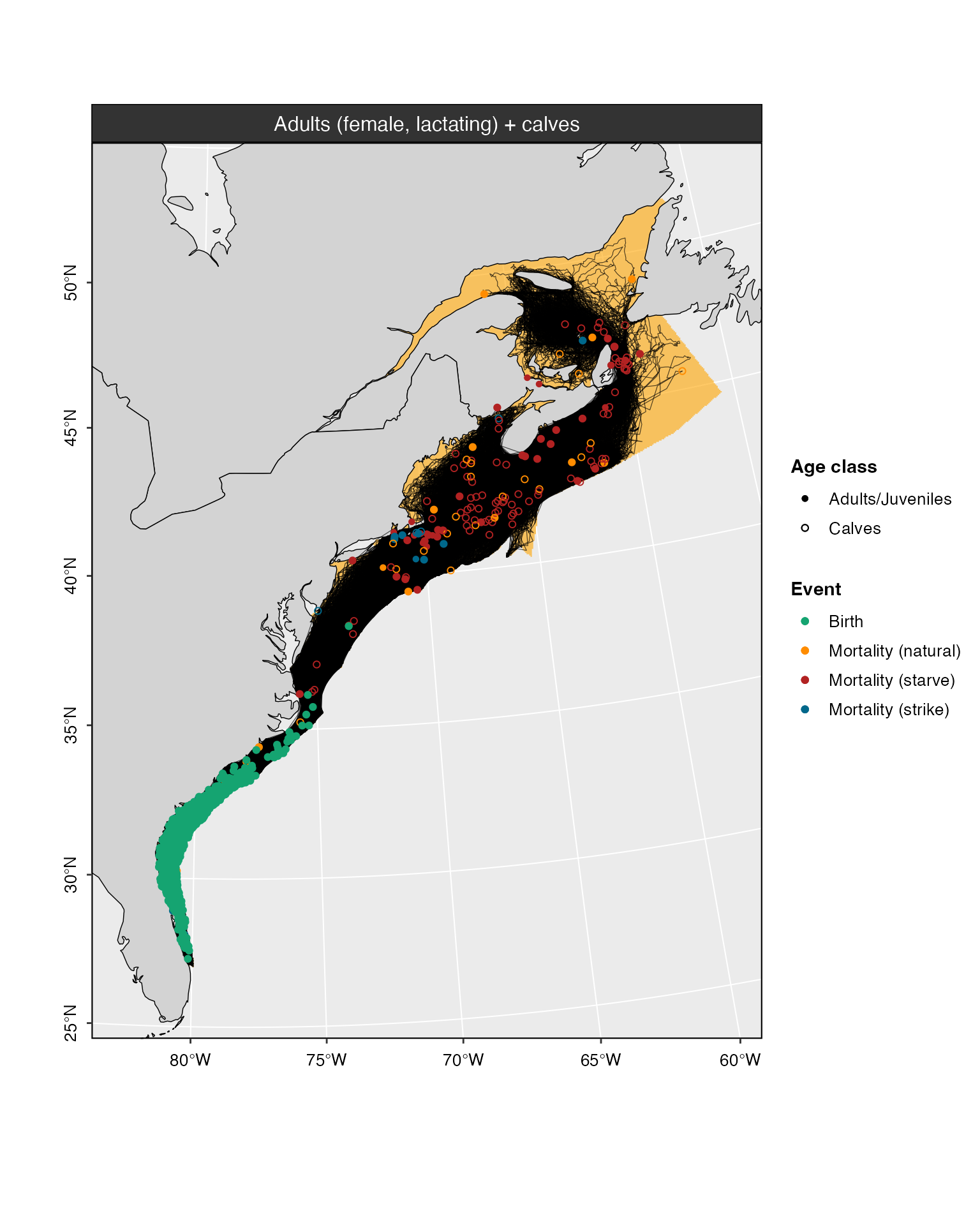
Plot aesthetics
The thickness and transparency of track lines can be changed via the
lwd and alpha arguments, respectively. Lower
values of lwd produce thinner lines, and lower values of
alpha increase transparency.
plot(model_base, cohort = 5, whale = 1:10, alpha = 0.2, lwd = 1)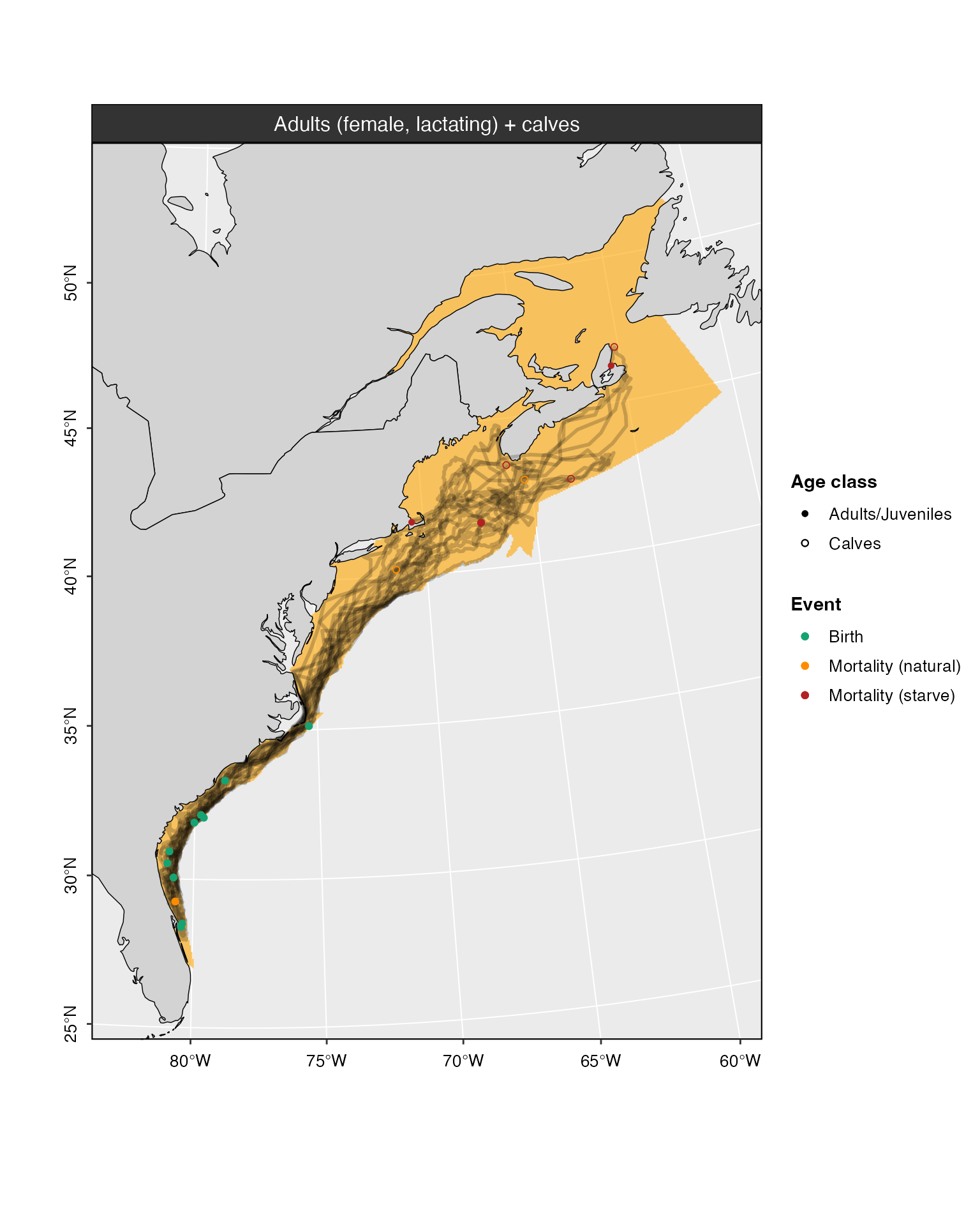
Interactive maps
Lastly, when web is set to TRUE,
interactive web-based maps are produced using the ggplotly R package.
These can be zoomed and panned using the mouse cursor to get a closer
look at specific areas of interest. The location (easting, northing) and
ID of each animal are displayed upon mouse hover.